Semiconductor

This is a place to get together a bunch of different analytical models and tabulated data sets for semiconductor properties. The main focus is Silicon, as that is what I work with.

All the models are implemented in a similar way. A class is built that allows switching between model written by different authors through the author command. The values calcualted are expected to be the same result in the values from the authors published implementation.

Examples

Here is an example of how to use calculate the band gap narrowing for silicon. We will look at two different band gap narrowing models. The default model is that from Yan in 2014. model.

    from semiconductor.material.bandgap_narrowing import BandGapNarrowing as BGN
    import numpy as np

    # initialise the class
    BGN_class = BGN(material='Si')
    # define the number of dopants
    Na = 0.
    Nd = np.logspace(16, 20)
    # Set the excess carriers to zero
    nxc = 0
    bgn_yan = BGN_class.update(Na=Na, Nd=Nd, nxc=nxc)

Other inputs for the bandgap narrowing class can be also found and set with the calculationdetails function:

  BGN_class.calculationdetails
  > {'Na':0.0,
     'Nd': array([  1.00000000e+16,   1.20679264e+16,   1.45634848e+16,
              1.75751062e+16,   2.12095089e+16,   2.55954792e+16,
              3.08884360e+16,   3.72759372e+16,   4.49843267e+16,
              5.42867544e+16,   6.55128557e+16,   7.90604321e+16,
              9.54095476e+16,   1.15139540e+17,   1.38949549e+17,
              1.67683294e+17,   2.02358965e+17,   2.44205309e+17,
              2.94705170e+17,   3.55648031e+17,   4.29193426e+17,
              5.17947468e+17,   6.25055193e+17,   7.54312006e+17,
              9.10298178e+17,   1.09854114e+18,   1.32571137e+18,
              1.59985872e+18,   1.93069773e+18,   2.32995181e+18,
              2.81176870e+18,   3.39322177e+18,   4.09491506e+18,
              4.94171336e+18,   5.96362332e+18,   7.19685673e+18,
              8.68511374e+18,   1.04811313e+19,   1.26485522e+19,
              1.52641797e+19,   1.84206997e+19,   2.22299648e+19,
              2.68269580e+19,   3.23745754e+19,   3.90693994e+19,
              4.71486636e+19,   5.68986603e+19,   6.86648845e+19,
              8.28642773e+19,   1.00000000e+20]),
     'author':None,
     'material':'Si',
     'nxc':0.0,
     'temp':300.0}
  BGN_class.calculationdetails = {nxc:nxc, temp:300}

If a different band gap narrowing model is desired, pick from the available ones. The available ones can be found using the available_models() function.

    print (BGN_class.available_models())

For the band gap narrowing function it returns.

    ['DelAlamo1985', 'Cuevas1996', 'Yan2013bz', 'Yan2014bz', 'Schenk1988fer', 'Schenk1988_reparamitisation_Yan2013', 'Yan2013fer', 'Yan2014fer']

Changing to a model by a different author is done using the author input in either the initalisation of the class, or through the "update" function. Lets choose Schenk's from 1988 and set it through the "update" function. All classes have a similar update function. If we look at the models inputs, we see it also needs an input for temperature. This is just passed to the update function, which passes it to the appropriate places.

    temp = 300
    bgn_sch = BGN_class.update(Na=Na, Nd=Nd, nxc=nxc, temp=300, author='Schenk1988fer')

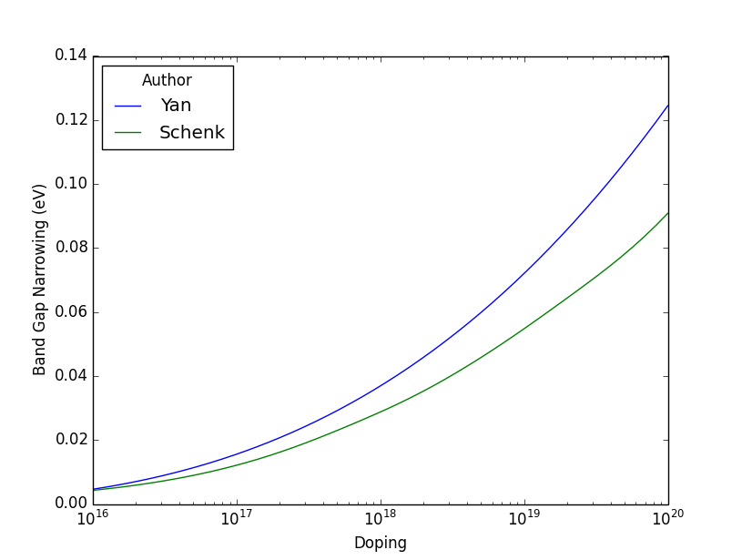
Finally we can plot, and compare the differences in the models.

    import matplotlib.pylab as plt

    plt.plot(Nd, bgn_yan, label = 'Yan')
    plt.plot(Nd, bgn_sch, label = 'Schenk')
    plt.legend(loc=0, title='Author')
    plt.xlabel('Doping')
    plt.ylabel('Band Gap Narrowing (eV)')
    plt.semilogx()
    plt.show()